072. Ordinary Least Squares Method (the line of best fit)
This method is called OLS because it results in line which is minimizes the squared vertical distances from each observation point to the line itself (Fig.7.3).

Figure 7.3 – Ordinary Least Squares
In Figure 7.3 Yi Is an actual, observed for the Y variable, Ŷ is a value on the line predicted by the equation.
Thus, the vertical difference between all the values Yi and Ŷ should be calculated and then squared to yield (Yi - Ŷ)2. All squared differences are summed then and expressed as
Σ(Yi – Ŷ)2 = min, (7.3)
Where Min is the number smaller than any summed squared vertical deviations between the actual data points and any other line. Hence, the term Least squares is used.
The difference Yi – Ŷ Is called Residual, or Error.
Assumptions of OLS.
1) The error term is a random variable and is normally distributed.
2) Any two errors are independent of each other, i. e. the error when Xi = 10 is totally independent of the error suffered when Xi+1 is equal to any other value.
3) All errors have the same variance. This condition is known as Homoscedastisity (Fig. 7.4).
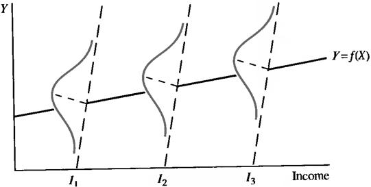
Figure 7.4 – Equality of Variance in the Error Term
4) The means of the Y – values all lie on a straight line. Given some value Xi, there will occur a normal distribution of Y-values. This distribution has a mean. The same is true if X is set equal to any other value. OLS assumes that these two means, as well as all others that might be observed, lie on a straight line. This is referred to as the assumption of linearity, and can be expressed as
![]() ,
,
Where ![]() is the mean of the population of Y-values for any given value of X.
is the mean of the population of Y-values for any given value of X.
To calculate the regression coefficient B0 And the intercept B1 in Formula (7.2B) the sums of squares and cross-products are used
 ,
, ![]() , (7.4)
, (7.4)
Where
![]() ,
,
 . (7.5)
These calculations are extremely sensitive to rounding. In the interest of accuracy it’s better to carry out calculations of five or six decimal places.
The meaning of b1: it indicates by how much Y will change for every one-unit change in the X-variable.
Example 7.4. In order to make decisions regarding allocations for the advertising budget, the accounting department for Hop Scotch Airlines must determine the nature of the relationship between advertising expenditures and the number of passengers. The senior accountant recognizes that regression analysis would be of invaluable assistance.
Table 7.2 – Regression Data for Hop Scotch Airlines
|
Observation (months) |
Advertising (in $1000’s) (X) |
Passengers (in $1000’s) (Y) |
XY |
X2 |
Y2 |
|
1 |
10 |
15 |
150 |
100 |
225 |
|
2 |
12 |
17 |
204 |
144 |
289 |
|
3 |
8 |
13 |
104 |
64 |
169 |
|
4 |
17 |
23 |
391 |
299 |
529 |
|
5 |
10 |
16 |
160 |
100 |
256 |
|
6 |
15 |
21 |
315 |
225 |
441 |
|
7 |
10 |
14 |
140 |
100 |
196 |
|
8 |
14 |
20 |
280 |
196 |
400 |
|
9 |
19 |
24 |
456 |
361 |
575 |
|
10 |
10 |
17 |
170 |
100 |
589 |
|
11 |
11 |
16 |
176 |
121 |
256 |
|
12 |
13 |
18 |
234 |
169 |
324 |
|
13 |
16 |
23 |
368 |
256 |
529 |
|
14 |
10 |
15 |
150 |
100 |
225 |
|
15 |
12 |
16 |
192 |
144 |
256 |
|
Total |
187 |
268 |
3490 |
2469 |
4960 |
Solution: from Formulas (7.4) coefficients of the regression model can be determined as
 or 1.08,
![]() or 4.4.
or 4.4.
The regression equation is therefore
Ŷ = 4.40 + 1.08X.
Interpretation:
1) The model tells that if, for example, $10000 is spent on advertising (X=10), then
Ŷ = 4.40 + 1.08(10) = 15.2 passengers (in 1000’s)
Will choose to fly Hop Scotch.
B) Since b1 = 1.08, for every additional $1000 that Hop Scotch spends on advertising, 1080 more passengers will choose this air company, i. e. if advertising is increased by one unit to $11000, the estimate of total passenger becomes Ŷ = 4.40 + 1.08(11) = 16.28 or 16280 passengers.
As there is no evidence of a cause – and – effect relationship the simultaneous increase in X and Y may have been caused by an unknown third variable excluded from the study. It is a common misconception to assume that there exists a cause – and – effect relationship between the two variables.
| < Предыдущая | Следующая > |
|---|